python
import numpy as np
import matplotlib.pyplot as plt

# 倒立摆参数
M = 1.0  # 小车质量 (kg)
m = 0.1  # 摆杆质量 (kg)
l = 0.5  # 摆杆长度 (m)
g = 9.81  # 重力加速度 (m/s²)


# 倒立摆动力学模型
def pendulum_model(state, F):
    x, x_dot, theta, theta_dot = state
    sin_theta = np.sin(theta)
    cos_theta = np.cos(theta)

    # 计算theta''
    numerator = (M + m) * g * sin_theta - F * cos_theta - m * l * theta_dot ** 2 * sin_theta * cos_theta
    denominator = l * (M + m - m * cos_theta ** 2)
    denominator = np.sign(denominator) * max(1e-6, abs(denominator))  # 避免除以零
    theta_ddot = numerator / denominator

    # 计算x''
    if abs(cos_theta) < 1e-6:
        cos_theta = np.sign(cos_theta) * 1e-6
    x_ddot = (g * sin_theta - l * theta_ddot) / cos_theta

    return np.array([x_dot, x_ddot, theta_dot, theta_ddot])


class ADRC:
    def __init__(self, dt, r, h, beta1, beta2, beta3, k1, k2, b0):
        self.dt = dt
        self.r = r
        self.h = h
        self.beta1 = beta1
        self.beta2 = beta2
        self.beta3 = beta3
        self.k1 = k1
        self.k2 = k2
        self.b0 = b0

        # 状态初始化
        self.v1 = 0.0
        self.v2 = 0.0
        self.z1 = 0.0
        self.z2 = 0.0
        self.z3 = 0.0
        self.u_prev = 0.0

    def fhan(self, x1, x2, r, h):
        d = r * h
        d0 = h * d
        y = x1 + h * x2
        a0 = np.sqrt(d ** 2 + 8 * r * np.abs(y))

        if np.abs(y) > d0:
            a = x2 + (a0 - d) / 2 * np.sign(y)
        else:
            a = x2 + y / h

        if np.abs(a) > d:
            return -r * np.sign(a)
        else:
            return -r * a / d

    def TD(self, target):
        e = self.v1 - target
        fh = self.fhan(e, self.v2, self.r, self.h)
        self.v1 += self.dt * self.v2
        self.v2 += self.dt * fh
        return self.v1, self.v2

    def ESO(self, y, u):
        e = self.z1 - y
        self.z1 += self.dt * (self.z2 - self.beta1 * e)
        self.z2 += self.dt * (self.z3 + self.b0 * u - self.beta2 * e)
        self.z3 += self.dt * (-self.beta3 * e)
        return self.z1, self.z2, self.z3

    def NLSEF(self, v1, v2, z1, z2):
        e1 = v1 - z1
        e2 = v2 - z2
        return self.k1 * e1 + self.k2 * e2

    def control(self, y, target):
        v1, v2 = self.TD(target)
        z1, z2, z3 = self.ESO(y, self.u_prev)
        u0 = self.NLSEF(v1, v2, z1, z2)
        u = (u0 - z3) / self.b0
        self.u_prev = u
        return u


# 仿真参数
dt = 0.001
sim_time = 5.0
t = np.arange(0, sim_time, dt)
n = len(t)

# 初始状态 (x, x_dot, theta, theta_dot)
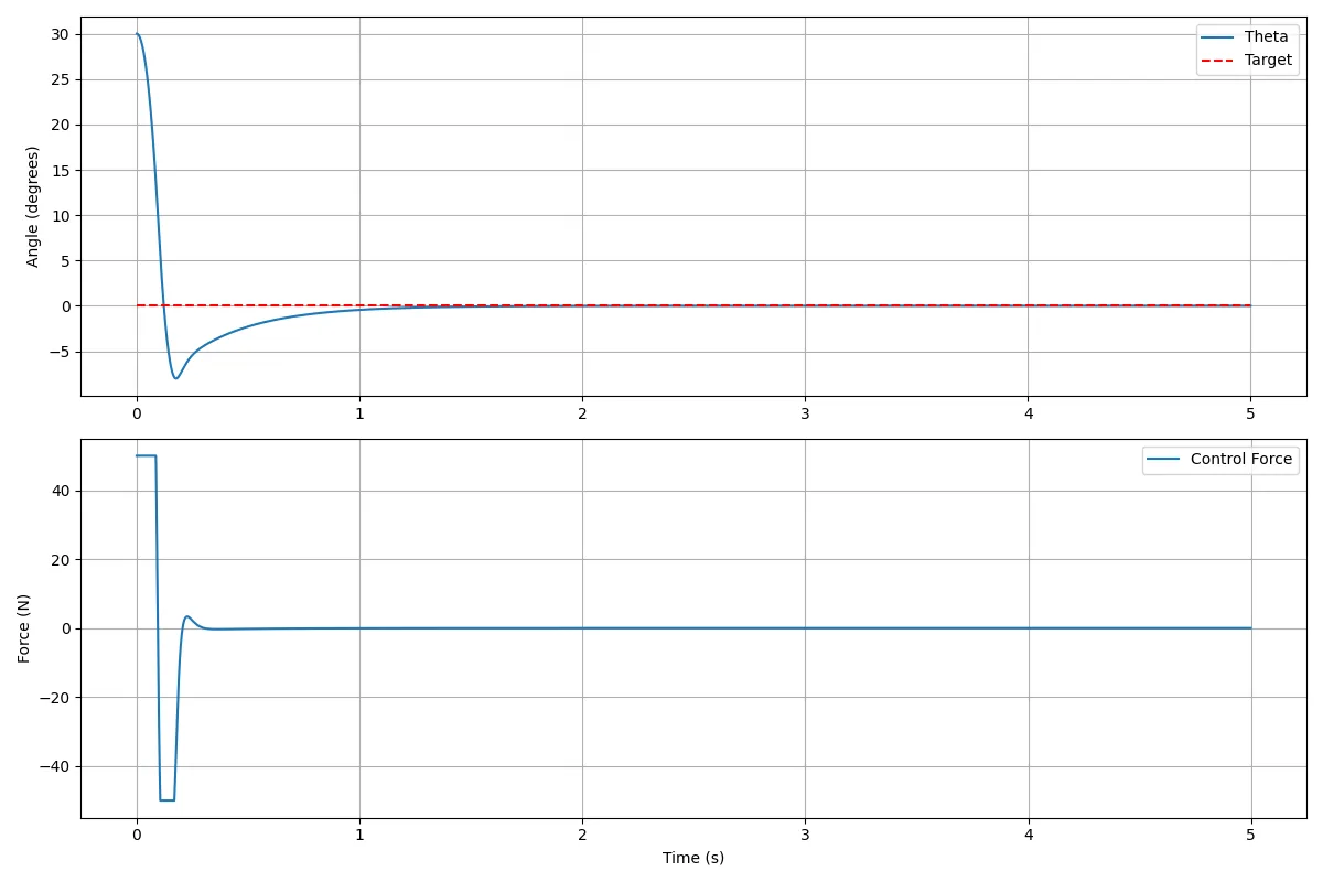
state = np.array([0.0, 0.0, np.pi / 6, 0.0])  # 初始角度30度

# ADRC参数
b0 = -1 / (l * M)  # 控制增益
adrc = ADRC(
    dt=dt,
    r=30,  # TD速度因子
    h=dt,  # TD滤波因子
    beta1=300,  # ESO参数 (3w)
    beta2=30000,  # (3w^2)
    beta3=1e6,  # (w^3)
    k1=150,  # NLSEF增益
    k2=50,
    b0=b0
)

# 初始化记录数组
states = np.zeros((n, 4))
F_history = np.zeros(n)
theta_history = np.zeros(n)

# 主循环
for i in range(n):
    # 获取当前角度作为系统输出
    current_theta = state[2]

    # ADRC控制
    F = adrc.control(current_theta, 0.0)
    F = np.clip(F, -50, 50)  # 限制控制力

    # 记录状态
    states[i] = state
    F_history[i] = F
    theta_history[i] = current_theta

    # 更新状态
    state_deriv = pendulum_model(state, F)
    state += state_deriv * dt

    # 角度归一化到[-pi, pi]
    if state[2] > np.pi:
        state[2] -= 2 * np.pi
    elif state[2] < -np.pi:
        state[2] += 2 * np.pi

# 绘图
plt.figure(figsize=(12, 8))
plt.subplot(2, 1, 1)
plt.plot(t, np.degrees(theta_history), label='Theta')  # 将弧度转换为度数
plt.plot([0, sim_time], [0, 0], 'r--', label='Target')
plt.ylabel('Angle (degrees)')  # 修改ylabel为度数
plt.legend()
plt.grid(True)

plt.subplot(2, 1, 2)
plt.plot(t, F_history, label='Control Force')
plt.ylabel('Force (N)')
plt.xlabel('Time (s)')
plt.legend()
plt.grid(True)

plt.tight_layout()
plt.show()